Building a Production Voice Agent: The Latency Budget Nobody Talks About
By Huzefa Motiwala · Co-Founder & Chief Product Officer
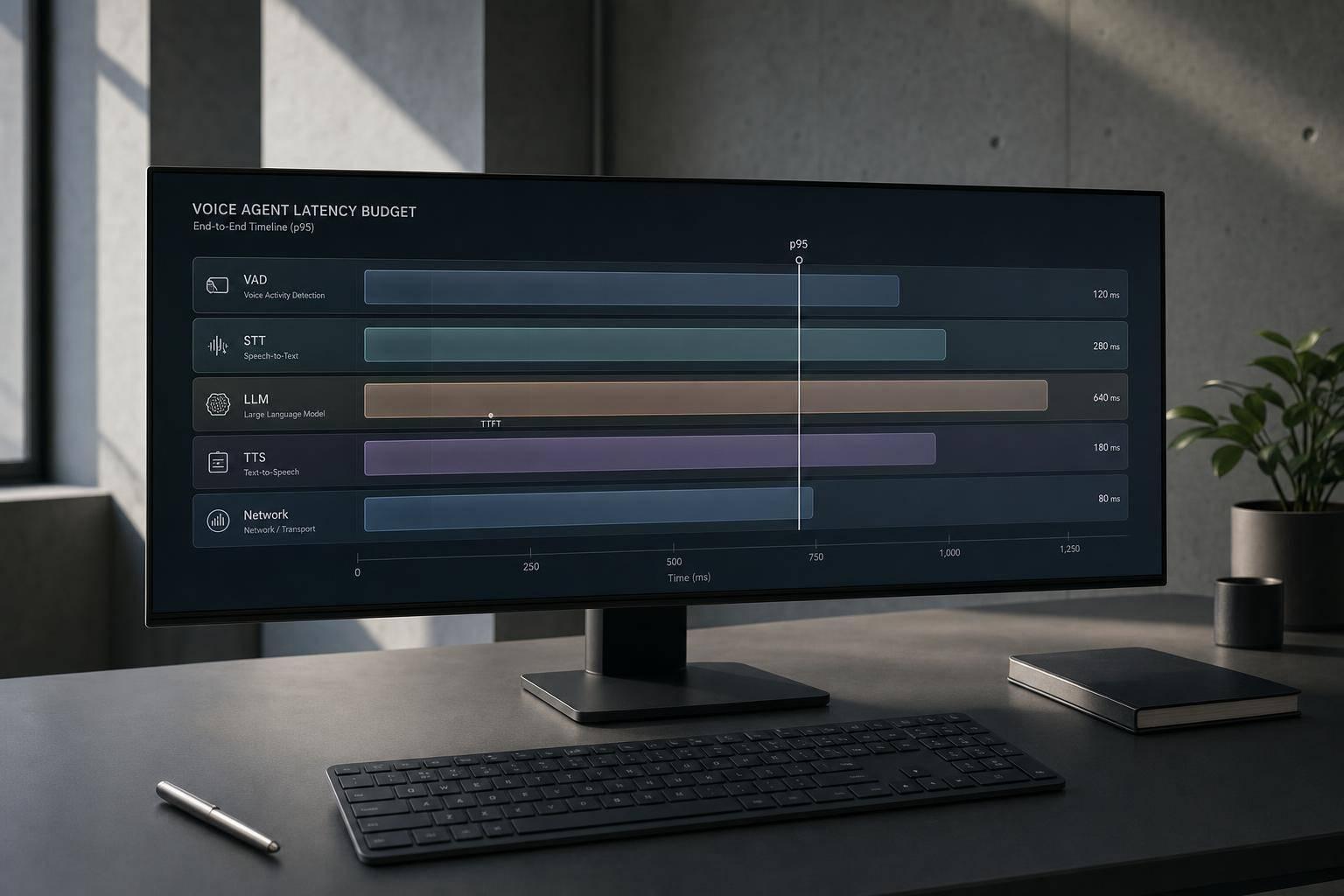
If your voice agent feels slow, the problem usually isn’t one model. It’s the whole path. What users feel is the gap between when they stop talking and when they hear the first reply. In practice, users start to notice lag at about 700 ms, may repeat themselves after 800 ms, and many calls feel broken at 1.5-2.0 seconds.
Here’s the short version:
- Latency is a budget across five parts: VAD, STT, LLM, TTS, and network.
- The main trouble spots are usually endpointing and LLM first-token delay.
- p95 matters more than p50. A system can look fine at 1.4 seconds p50 and still feel bad at 3.4 seconds p95.
- Streaming cuts perceived delay. Instead of waiting for each step to finish, the best systems overlap STT, LLM, and TTS.
- Network and jitter are easy to miss. Even a good setup can lose 20-50 ms each way, plus buffer time.
If I had to boil the article down to one point, it would be this: treat latency like a fixed budget, measure it by stage, and design around p95 - not demo averages.
A few numbers shape the whole system:
- Human turn gaps average about 200 ms
- A usable target is often ~800 ms p95
- Endpointing alone can cost 300-800 ms
- LLM TTFT can move from 566 ms p50 to 2,246 ms p95
- PSTN paths can add a 600 ms+ floor before model time even starts
So when I build or review a voice stack, I focus on three things first:
- Cut end-of-turn wait time
- Lower LLM time-to-first-token
- Keep every stage streaming and in the same region when possible
This article is a guide to where the milliseconds go, what makes them grow, and how to keep the full system inside a turn-time budget that users can tolerate.
Reduce the Latency of your Voice Agent
The production voice pipeline and its latency budget
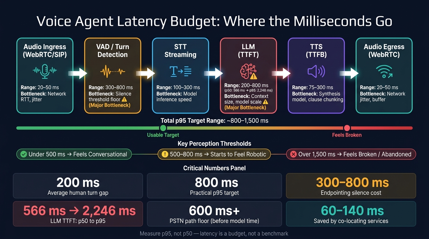
Voice Agent Latency Budget: Where the Milliseconds Go
Every production voice agent burns time in the same chain: audio in, VAD, STT, LLM, TTS, and audio out. Each step takes a slice of the budget. The catch is that teams often don’t look at the full path together until the system starts to feel slow in production.
Stage-by-stage breakdown: VAD, STT, LLM, TTS, and network
Network transport usually adds 20 ms-50 ms each way, plus jitter [2][7]. After that, Voice Activity Detection (VAD) splits speech from background noise in about 10 ms-50 ms of compute time [2].
But here’s where things often drag: endpointing tends to cost more than VAD compute itself. Many systems wait for 300 ms to 800 ms of silence before they decide the user is done speaking [7]. That alone can eat up most of the budget before STT even gets moving.
Once the turn is detected, streaming STT starts turning audio into text. The metric to watch is first partial transcript latency, not final transcript completion. That early partial - often available every 100 ms-250 ms - can kick off the next stage before the user has fully stopped talking [7].
The LLM stage is tracked with Time-to-First-Token (TTFT), which is the moment the first token of the reply shows up. This is often the shakiest part of the pipeline. In production traces, TTFT can shift from 566 ms at p50 to 2,246 ms at p95 as conversation history gets longer [1].
Then streaming TTS begins generating audio from the first chunk of the reply. This is measured with Time-to-First-Byte (TTFB), while the rest of the text is still streaming in [2][7]. That overlap matters a lot. With streaming, latency starts to look more like the slowest stage than the total of every stage added together.
Budget table: where the milliseconds go
| Pipeline Stage | Documented Range | Primary Bottleneck |
|---|---|---|
| Audio Ingress (WebRTC/SIP) | 20 ms - 50 ms | Network RTT, jitter |
| VAD / Turn Detection | 300 ms - 800 ms | Silence threshold floor |
| STT (Streaming, first partial) | 100 ms - 300 ms | Model inference speed |
| LLM (TTFT) | 200 ms - 800 ms | Context size, model scale |
| TTS (TTFB, first audio chunk) | 75 ms - 300 ms | Synthesis model, clause chunking |
| Audio Egress (WebRTC) | 20 ms - 50 ms | Network jitter, buffer |
These numbers are the budget. And two levers stand out right away: endpointing and LLM TTFT. Endpointing gives you the most room to tune, while TTFT brings the ugliest tail, climbing from 566 ms to 2,246 ms as context grows [1].
What drives latency at each stage and how to cut it
The table above shows where the milliseconds go. This section gets into the knobs that change them. Each stage has its own main source of delay, so it makes sense to fix the worst bottleneck first.
VAD and STT: endpointing, partial transcripts, and service placement
A fixed-silence endpointer can burn 500 ms or more just waiting before it decides the speaker is done. That’s dead air. Model-based endpointing does better because it uses acoustic and semantic cues, and it can fire in about 200-400 ms. In practice, that can win back 250-350 ms from the turn budget without changing the rest of the stack [6][4].
Streaming STT also matters. It can produce the first word in about 90 ms [6]. And if the LLM doesn’t need polished text, turn off formatting like punctuation and capitalization. That skips extra processing and trims delay [8].
Where your services run matters too. Cross-region hops between STT, LLM, and TTS can add about 60-140 ms of round-trip time. Putting those services together at the media edge cuts those hops and keeps the pipeline tighter [6][5].
Once turn detection gets fast, the next bottleneck is usually model turn time.
LLM and TTS: first token, first audio chunk, and streaming handoff
LLM TTFT is often the biggest swing factor. Prompt size, context length, and sequential tool calls all push it higher [4][1][5]. A few practical levers help:
- Use prompt caching
- Pick smaller non-reasoning models for the live turn
- Limit tool steps
- Keep the live voice path on low-latency models
- Save high-reasoning models for offline steps [6]
TTS should start on the first clause, not after the whole sentence. Waiting for a full sentence or paragraph can cost 300-800 ms. If synthesis starts as soon as the first clause arrives, audio generation can overlap with the rest of the LLM response [6][8].
After model and synthesis tuning, transport often becomes the hidden cost.
Network and jitter: the hidden cost in real-time systems
WebRTC usually adds about 100 ms of network overhead when servers are placed well. PSTN and telephony paths are much heavier, with a 600 ms+ floor because of carrier routing, signaling, and codec transcoding [8]. If phone calls are part of your use case, that floor needs to be built into your p95 target.
Cold HTTP connections can add another 100-200 ms because of TLS handshakes, which is why persistent keep-alive connections matter [7]. Adaptive jitter buffers like WebRTC’s NetEQ add a 30-120 ms stability tax. Still, that trade-off is usually worth it, since they deal with packet loss without stalling playback [6]. Keep round trips low, keep services in one region, and use a transport built for live audio.
Use these levers to set your p95 targets in the next section.
How to build a latency budget for your own architecture
A step-by-step method for setting p95 targets
Start with transport. Set aside its floor before you assign time to compute. That floor tells you how much room is left for VAD, STT, LLM, and TTS.
Then work backward from your p95 end-to-end target. Human perception gives you a useful guardrail here: under 500 ms feels conversational, over 800 ms starts to feel robotic, and past 1,500 ms feels broken [4][6]. An 800 ms p95 target is a practical place to begin. Subtract the transport floor, then divide what remains across the compute stages.
In a streaming pipeline, total latency is driven by the slowest stage, not the sum of every stage. That’s the rule of thumb to use when you split your p95 target across the stages below.
After you allocate transport, find the compute stage with the highest and most volatile p95. In many cases, that’s LLM TTFT. Make that your first fix [3][1]. Give STT and TTS tighter budgets, and reserve 30-150 ms for jitter and adaptive buffering. Use a larger network allowance only if ingress, egress, and service hops are all in the path.
Think of this as a worksheet for your own measured p95s, not a fixed benchmark. The split will change based on model choice, co-location, and whether you stream at sentence boundaries.
| Stage | Illustrative p95 Budget | Primary Lever |
|---|---|---|
| Network (uplink/ingress) | 100-150 ms | WebRTC, regional co-location |
| VAD / Endpointing | 200-400 ms | Semantic/model-based detection |
| STT (finalization) | 50-250 ms | Streaming partials, integrated end-of-turn |
| LLM (TTFT) | 200-700 ms | Fast non-reasoning models, prompt caching |
| TTS (TTFB) | 50-350 ms | Flash-class models, persistent WebSockets |
| Buffering / Jitter | 30-150 ms | Adaptive jitter buffers |
| Total Target (p95) | ~800-1,500 ms | Streaming and overlapping stages |
A gap table: current state vs. target state
Once you have a target allocation, measure where you are now. Instrument each stage so you capture p95 spans, not averages, with observability tooling that records individual turn traces [5][9]. Then fill in a gap table.
The format is simple: Stage | Current p95 | Target p95 | Gap | Architectural Lever. The gap column tells you what to fix next. Start with the largest gap. If endpointing has the biggest miss, that usually points to moving from fixed-silence detection to semantic VAD [4][6][3]. If the main issue is LLM TTFT, look at a faster non-reasoning model or a lower-latency inference path [6][3].
| Stage | Current p95 | Target p95 | Gap | Architectural Lever |
|---|---|---|---|---|
| Endpointing | ___ ms | ___ ms | ___ ms | e.g., Switch from fixed silence to semantic VAD |
| LLM (TTFT) | ___ ms | ___ ms | ___ ms | e.g., Use smaller/distilled model or faster inference |
| TTS (TTFB) | ___ ms | ___ ms | ___ ms | e.g., Switch to a flash-class TTS model |
| Network | ___ ms | ___ ms | ___ ms | e.g., Co-locate agent with model inference region |
| LLM→TTS handoff | ___ ms | ___ ms | ___ ms | e.g., Implement streaming between LLM and TTS |
Run this audit before launch and again after major changes. Use the gap table to define the monitors in the next section.
Production hardening: treat latency as a monitored system constraint
Once you set the budget, protect it in production. That’s where the hard part starts.
Latency drifts after launch as prompts change, context gets longer, tools get added, and cold starts show up at the worst time. So don’t treat latency like a one-time benchmark. Treat it like a budget with clear thresholds, alerts, and a named owner.
What to measure after launch
Use the same stages from your budget table in your runtime dashboard. For each turn, trace four spans:
- endpointing delay
- LLM TTFT
- TTS time to first audio chunk
- network egress time
If you only log end-to-end latency, you’re flying blind. You’ll know something got slower, but not where it happened.
Track p95 for each span. Use p50 as a baseline, not the main signal. Then connect those spans to token counts, conversation depth, and specific tool calls. That makes it much easier to see whether a slowdown is coming from the model, the agent layer, or transport.
Set alerts for gaps above 10 ms between stages, and put timeouts around LLM calls and tool work. If a turn is going to run long, play a short filler sound or acknowledgment instead of leaving dead air. Users notice delays past 500 ms, and abandonment spikes beyond 1,500 ms [7][4].
Key takeaways for founders and technical leaders
The rule is simple: measure the same spans you budgeted, then react when p95 starts drifting.
Run your gap table again after any prompt update, model swap, region change, or tool integration. Keep the agent, STT, LLM, and TTS in the same region whenever you can to cut inter-service latency. And when p95 spikes, don’t brush it off as noise. Treat it as a sign that something in the architecture changed.
FAQs
How do I set a realistic latency budget?
Set your target around total time-to-first-audio (TTFA). That’s the time from the moment a user stops speaking to the moment they hear the first bit of your reply.
The big idea is simple: don’t treat this as one long, blocking chain. In production, parts of the pipeline can stream and overlap. If you budget each stage as if every step has to wait for the last one to finish, your latency math will be off.
A practical production target is under 1 second end to end. If you’re pushing hard, around 300 ms is the kind of stretch goal teams aim for.
Also, don’t just stare at averages. Watch P95 performance. That’s where the rough edges show up, and it’s often what users remember. On top of that, trim end-of-turn delay with semantic turn detection instead of fixed silence thresholds. Fixed thresholds are blunt; semantic detection is better at spotting when someone is actually done talking.
What should I optimize first in a voice pipeline?
First, add observability so you can see where the delay is coming from: STT, LLM, or TTS.
Then go after the biggest wins:
- Endpointing: tighten silence thresholds or use semantic turn detection
- Co-location: keep services in the same cloud region
- Streaming: stream end to end
- Faster models: use them if the LLM is the bottleneck
Why does p95 matter more than average latency?
Average latency (P50) can paint too rosy a picture for production voice agents. It smooths over the random slowdowns that users actually notice, and those are often the moments that make an interaction feel clunky.
P95 tells a much more useful story. It shows the slower cases, like network jitter, complex tool calls, or long-context LLM processing. And those slower moments are often what decide whether the agent feels responsive or frustratingly laggy.
Related Blog Posts
- Voice Agent Latency: Where the 2-3 Second Delay Actually Lives in the Pipeline and How to Reduce It
- Why VAD End-of-Speech Detection Is the Hardest Problem in Production Voice Agents
- Multi-Language Voice Agent Architecture: How We Structure Prompts and Fallbacks Across 8 Languages
- Why Most Agent Framework Benchmarks Don’t Predict What Happens in Production