Voice Agent Latency: Where the 2–3 Second Delay Actually Lives in the Pipeline and How to Reduce It

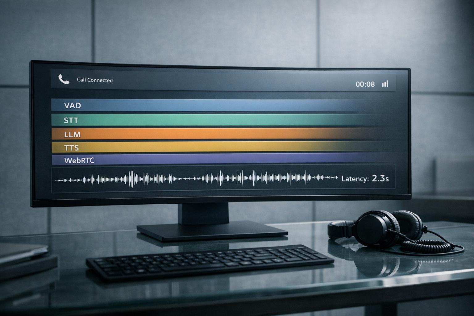
Latency is the biggest frustration in voice agents. A 2–3 second delay between when a user stops speaking and the agent starts responding feels unnatural and disrupts conversations. Here’s why it happens and how to fix it:

• Key delay contributors:
  • Voice Activity Detection (VAD): 300–800ms
  • Speech-to-Text (STT): 150–500ms
  • Large Language Model (LLM): 200–800ms
  • Text-to-Speech (TTS): 100–500ms
  • Network: 50–200ms
• Solutions to reduce delays:
  • Use streaming architectures to overlap processes.
  • Lower VAD silence thresholds (e.g., 200–400ms).
  • Optimize STT and LLM models for faster processing.
  • Implement streaming TTS for quicker audio playback.
  • Minimize network overhead with WebRTC and regional deployments.

Reduce the Latency of your Voice Agent

sbb-itb-51b9a02

The Voice Agent Pipeline: Where Time Gets Lost

Your voice agent operates through five key stages, each contributing to the overall delay. Knowing where time is spent allows you to focus on precise optimizations rather than relying on guesswork.

Pipeline Stages and Latency Ranges

Every interaction flows through VAD (Voice Activity Detection), STT (Speech-to-Text), the LLM (Large Language Model), TTS (Text-to-Speech), and network transport.

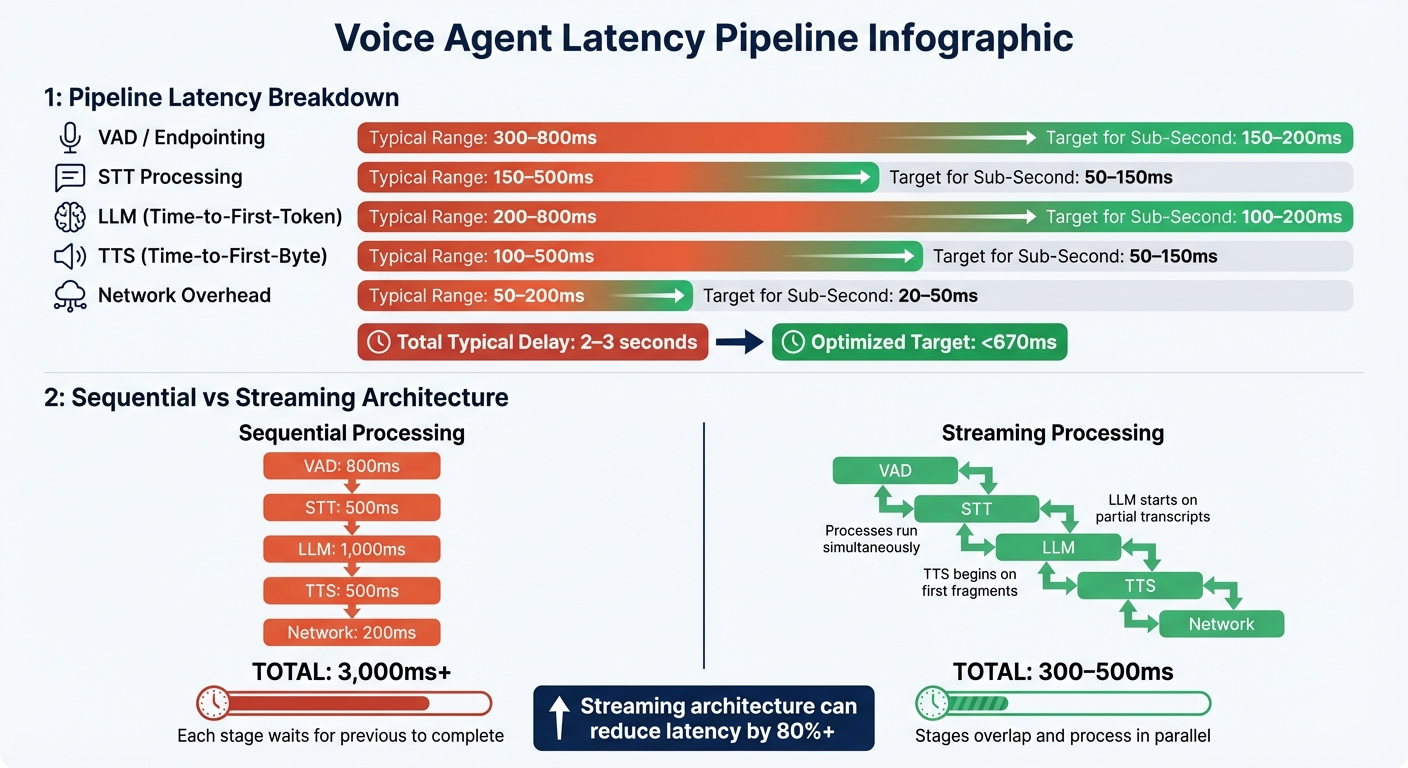
Here’s a closer look at how a typical 2–3 second delay breaks down:

Pipeline Stage	Typical Range	Target for Sub-Second
VAD / Endpointing	300–800ms	150–200ms
STT Processing	150–500ms	50–150ms
LLM (Time-to-First-Token)	200–800ms	100–200ms
TTS (Time-to-First-Byte)	100–500ms	50–150ms
Network Overhead	50–200ms	20–50ms

VAD endpointing often accounts for the largest delay. While VAD processing itself is nearly instantaneous, systems typically wait for 300–800ms of silence to confirm the end of speech ^[1].

Another major factor is the LLM’s Time-to-First-Token (TTFT). For instance, switching from GPT-4 Turbo to GPT-4o-mini in production telephony environments reduced median TTFT from about 2.8 seconds to 0.9 seconds ^[10]. However, as conversation history grows, P95 TTFT values can still exceed 2.2 seconds ^[6].

Network transport also adds delays. Standard cloud round-trips contribute 50–200ms, while WebRTC can lower this to 20–50ms ^[2][4]. On the other hand, traditional PSTN telephony can introduce an additional 150–700ms due to carrier routing ^[4].

These latency insights provide a foundation for comparing sequential and streaming processing approaches.

Sequential vs. Streaming Processing

After mapping out the latency contributions, it’s clear that processing architecture plays a huge role in overall delay.

In a sequential architecture, each stage waits for the previous one to finish. For example, the system first collects your full utterance, completes the STT, generates the entire LLM response, synthesizes the full audio, and finally plays it back. This stacking of delays – such as 800ms for VAD, 500ms for STT, 1,000ms for LLM, 500ms for TTS, and 200ms for network transport – can easily add up to 3 seconds or more ^[2][4].

In contrast, streaming architectures overlap these stages. The LLM begins processing partial transcripts while you’re still speaking, and TTS starts synthesizing audio as soon as the first fragment is ready. This parallel approach can cut total perceived latency to 300–500ms ^[11][4].

A real-world example highlights the impact of targeted optimizations. In March 2026, AI backend engineer Mohd Mursaleen improved Claritel’s voice agent by addressing specific latency components. Switching to streaming TTS shaved off 1.1 seconds, fine-tuning the LLM context and adopting GPT-4o-mini saved 2.2 seconds, and lowering the VAD silence threshold from 800ms to 400ms reduced another 400ms. These changes boosted call completion rates from 61% to 89% ^[10].

"Streaming architecture is not optional… the single biggest latency optimization in voice AI is not model selection, hardware, or network routing. It’s eliminating sequential waiting." – Tianpan.co ^[4]

The most critical measure for streaming systems is perceived latency – the silence between when you stop speaking and when the agent starts responding. This includes the end-of-utterance delay, LLM TTFT, and TTS time-to-first-byte ^[6], all of which occur simultaneously in a streaming setup.

Component-by-Component Latency Analysis

Now that you’re familiar with the pipeline architecture, let’s take a closer look at each component. Understanding the sources of latency, configuration options, and trade-offs can guide you in making smarter optimization choices.

VAD End-of-Speech Detection

While VAD (Voice Activity Detection) processing itself is nearly instantaneous, the silence threshold introduces some delay. Lowering this threshold can help reduce latency. For fast-paced interactions, like transactional agents, a threshold of 200–250ms works well. On the other hand, systems like appointment scheduling might benefit from a slightly higher threshold of around 400ms^[9].

Advanced systems like ML-based VAD (e.g., Silero) or semantic turn detection (e.g., Deepgram Flux) can cut endpointing delays to as low as 150–200ms. These systems analyze pitch, energy, and even lexical signals, rather than just silence^[2][4]. Plus, semantic endpointing reduces false interruptions by about 45% compared to traditional VAD-only setups^[4].

The trade-off here is balancing speed and accuracy. Lower thresholds might cut users off prematurely, while higher thresholds could feel sluggish. As Pradeep Jindal from ByondLabs puts it:

"Don’t disable smart features when they cause latency. Tune their sensitivity way down instead"^[3].

Next, let’s see how transcription methods influence overall latency.

STT Transcription Latency

Streaming STT processes audio in real time, delivering partial transcripts as the user speaks. This allows the LLM to start processing before the user even finishes. In contrast, batch STT waits for the full utterance before transcribing, adding extra delay. To speed things up, you can disable optional features like punctuation, filler word detection, and numeral conversion^[3][5].

Using quantized models like Whisper Tiny INT8 can reduce inference times by 40–60% on mobile devices^[1]. However, this may slightly compromise transcription accuracy. The key trade-off is clear: streaming STT provides faster responses but might sacrifice some polish in the transcript.

Once transcription is optimized, the next hurdle is minimizing LLM token generation delay.

LLM First-Token Latency

Time-to-First-Token (TTFT) often accounts for the biggest delay in the pipeline. Optimized models, such as Groq-hosted Llama variants, can achieve TTFT as low as 50–150ms. In contrast, less optimized or larger-context models may average 2–3 seconds, with P95 values sometimes exceeding 2.2 seconds^[2][4].

Efficient prompt engineering plays a big role here. Reducing or summarizing conversation history helps keep the prompt size manageable, as larger context windows significantly increase TTFT^[6][9]. Geographic co-location of servers and model providers can shave off 150–200ms^[7]. Techniques like LLM hedging – sending parallel requests to multiple providers and using the fastest response – can also reduce P99 latency^[2][4]. However, smaller models might respond faster but are less equipped for complex reasoning.

TTS Generation and Streaming Start

Time-to-First-Byte (TTFB) measures how quickly the user hears the first audio frame. Standard neural TTS systems take around 300ms or more, but optimized systems like Cartesia Turbo can bring this down to 40ms^[2][9]. With streaming TTS, playback starts as soon as the first sentence fragment is ready, overlapping TTS generation with LLM token generation. This significantly reduces perceived latency^[4].

The downside? Audio completeness. If the LLM changes direction mid-response or if the user interrupts, the system might need to cancel partially played audio and clear the queue within milliseconds^[4]. Ensuring smooth barge-in handling – where TTS stops immediately when a user interrupts – is critical.

Network Round-Trip Costs

Network transport adds anywhere from 40–200ms of latency, depending on the setup^[2][4]. WebRTC offers low-latency transport with round-trip times of 20–50ms, whereas traditional PSTN telephony introduces 150–700ms due to carrier routing^[2][4]. Cross-region network calls can add 50–100ms per trip, and with multiple calls per interaction, delays can stack up to 600ms^[2].

Using persistent connections – via WebSockets or gRPC with keep-alive and DNS caching – can reduce latency by avoiding repeated TCP handshakes. Co-locating components and deploying regional inference also helps minimize delays^[2][4]. The trade-off? Increased infrastructure complexity and costs, as edge deployments and regional redundancy demand more resources.

How to Measure and Isolate Latency Bottlenecks

Reducing latency begins with measuring it accurately. To address latency issues, you need to pinpoint where delays are occurring in your deployment. As Pradeep Jindal from ByondLabs aptly states:

"If you can’t produce a per-turn latency log for every single turn, you’re tuning blind." ^[3]

Measurement Protocol

Start by adding timestamps to every stage of your pipeline. Record the exact moments when the VAD (Voice Activity Detection) triggers the end-of-utterance (EOU), the STT (Speech-to-Text) completes transcription, the LLM (Large Language Model) delivers its first token (TTFT), and the TTS (Text-to-Speech) sends its first audio byte (TTFB). Instead of focusing solely on total round-trip time, you need granular, component-level data to identify the bottleneck ^[12].

Leverage tools like OpenTelemetry to create nested spans for detailed visibility across each component ^[14]. For network diagnostics, tools such as Deepgram’s network_latency can dissect processes like DNS resolution, TCP connection, TLS handshake, and WebSocket upgrades ^[13]. Once you’ve collected detailed timestamps, analyze the data to locate specific latency issues. Keep in mind that tracking each turn individually is crucial, as cold starts and outliers can distort average measurements.

The formula for perceived latency is: EOU Delay + LLM TTFT + TTS TTFB ^[6]. This represents the silence between when a user stops speaking and when the system begins responding.

Analyzing Latency Data

With your data in hand, carefully evaluate the latency breakdown. Averages can often be misleading. For instance, a 300ms average might mask the fact that 90% of users experience only 150ms, while 10% endure 1,500ms delays. Focusing on P95 and P99 percentiles is essential, as these metrics spotlight "tail latency", which frequently causes users to abandon interactions [14, 16].

In March 2026, Diego Fernando Valle Ortiz conducted a test using a stack that included Deepgram Nova 3, Ministral 3B, and Pocket TTS over 36 turns. The results revealed a P50 perceived latency of 1,392ms, while the P95 climbed to 3,384ms. The main culprit? An increase in LLM TTFT – from 566ms at P50 to 2,246ms at P95 – as conversation history expanded ^[6]. Such detailed analysis is vital for directing optimization efforts where they’re needed most.

To understand latency distribution, use histogram buckets: 50ms intervals for the 0–500ms range (the natural conversation threshold) and 250ms intervals for the 1,000–3,000ms range (where users are likely to abandon interactions) ^[14]. Latencies under 500ms feel seamless, delays between 500–800ms are tolerable for many business applications, but delays exceeding 1,200ms often lead to user frustration, prompting them to repeat themselves or hang up ^[9]. Additionally, every extra second of latency can reduce user satisfaction by 15–20%, while delays over 3 seconds can push abandonment rates above 40% ^[12].

Conclusion

Voice agent latency stems from a series of interconnected processes that can leave users waiting in silence. Without optimization, this delay can easily exceed 3,300ms. However, with a fine-tuned system, responses can be delivered in under 670ms ^[9][5]. Achieving this requires pinpointing inefficiencies and making calculated trade-offs between speed, quality, and cost.

As Pradeep Jindal from ByondLabs explains:

"Latency in voice agents is not about any single component. It’s about the orchestration between them." ^[3]

This highlights the importance of a holistic approach to achieving sub–2‑second latency. A key strategy is moving from sequential to streaming architectures, which allows overlapping of STT, LLM, and TTS processes. This shift alone can cut over a second of perceived delay ^[2][4]. Other trade-offs include choosing faster models, such as Groq-hosted Llama variants (50–150ms TTFT), over more advanced models like GPT-4o (200–800ms TTFT); fine-tuning VAD for faster response (200–400ms silence thresholds) versus using semantic turn detection; and prioritizing speed-optimized TTS (40–90ms TTFB) over higher-quality synthesis (200–400ms TTFB) ^[7][2][8].

Precise per-turn latency logs are critical for effective optimization. Focus on P95 and P99 percentiles rather than averages, as users are most affected by tail latency ^[4][5][2]. To shave off additional milliseconds, co-locate infrastructure with your telephony provider, pre-warm connections, and disable unnecessary STT flags ^[8][9][3].

Every optimization decision – whether balancing model speed with reasoning depth, VAD sensitivity with user experience, or TTS speed with audio quality – requires careful adjustment. The right balance depends on your use case, whether it’s a customer service agent handling complex issues or a conversational assistant where speed is the top priority. Detailed latency logs should guide these decisions, enabling CTOs and engineers to target improvements that make a tangible difference in voice agent performance.

FAQs

What should I log per turn to pinpoint latency?

To measure latency per turn in a voice agent, it’s important to log the timing of each step in the pipeline. Key components to track include:

• End-of-utterance detection time (VAD): How long it takes to detect when the user has finished speaking.
• Speech-to-Text (STT) processing time: The duration required to convert spoken words into text.
• LLM inference time: The time spent generating a response using the language model.
• Text-to-Speech (TTS) generation time: Includes both the time to create the audio and when streaming begins.
• Network round-trip times: The delay caused by data traveling to and from the server.
• Response start time: When the system begins delivering the response to the user.

By analyzing these logs, you can identify which component is slowing things down and focus on improving that specific area.

How can I cut VAD endpointing delay without cutting users off?

To minimize Voice Activity Detection (VAD) endpointing delay while ensuring users aren’t interrupted, fine-tune the VAD sensitivity to accommodate natural pauses in speech. Steer clear of overly strict silence thresholds, as they can lead to premature cut-offs. Incorporating model-based turn detection can enhance accuracy and maintain smoother interactions. Continuously monitor and evaluate pipeline delays to pinpoint the right areas for adjustment without disrupting the flow of the conversation.

What’s the fastest way to reduce LLM time-to-first-token as context grows?

To make large language models (LLMs) respond faster as the context size increases, consider implementing a sentence-streaming architecture. This approach allows token generation to begin even before the entire response is fully processed. The result? A noticeable reduction in perceived latency – by as much as 40–60%.

In addition to sentence-streaming, you can further improve response times by:

• Optimizing inference models: Use models designed for faster processing.
• Shortening input prompts: Streamlining the input can reduce processing overhead.

Among these strategies, sentence-streaming tends to have the most immediate and substantial effect, especially when dealing with larger contexts.

Related Blog Posts

• LangGraph vs CrewAI vs AutoGen: How We Evaluated All Three Before Recommending One for a Production Deployment